Planaria single-cell
This section uses data from the paper Plass et al., 2018. It contains expression levels of \(p= 5821\) genes measured across \(n=5000\) individual cells from adult planarians, a type of flatworm. Such data offer the possibility of discovering the cell lineage tree of an entire animal: the aim is to find out if the data reflect the tree-structured process by which stem cells differentiate into a variety of distinct cell types. These data were prepared using the Python package Scanpy, where the script on how to do this can be found here.
Load data
data = eb.load_planaria()

Y = data['Y']
labels = data['labels']
ordered_cats = data['cell_types']
colors = data['color_dict']
Data loaded successfully
(n,p) = Y.shape
print('Data matrix is', n, 'samples by', p, 'features')
Data matrix is 5000 samples by 100 features
Dimension selection and visualisation
After selecting the dimension Whiteley et al., 2022, perform PCA with embedding function and visualise.
ws, dim = eb.wasserstein_dimension_select(Y, range(40), split=0.5)
print("Selected dimension: {}".format(dim))
100%|██████████| 40/40 [01:06<00:00, 1.67s/it]
Recommended dimension: 16, Wasserstein distance 0.18280
Selected dimension: 16
zeta = eb.embed(Y, d=14, version='full')
## TSNE
from sklearn.manifold import TSNE
tsne = TSNE(n_components=2, perplexity = 30).fit_transform(zeta)
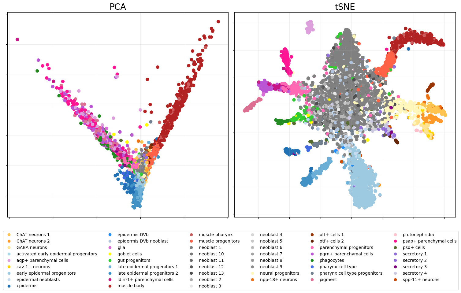
We can plot the two representations of our data with the
snapshot_plot function.
pca_fig = eb.snapshot_plot(
    embedding = [zeta[:,:2],tsne],
    node_labels = labels.tolist(),
    c = colors,
    title = ['PCA','tSNE'],
    add_legend=True,
    max_legend_cols = 6,
   figsize = (15,7.5),
   move_legend= (.5,-.3),
    # Apply other matplotlib settings
    s=50,
)
plt.tight_layout()

Construct tree
From here we want to perform hierarchical clustering on the data and simplify this tree. This can be done using the hierarchical clustering module.
We use hierarchical clustering with dot products as descibed in Gray et
al.,
2024.
This is the default HC in the class ConstructTree so we can just
give it our point cloud. Otherwise, the HC can be done first and the
model can be given to the ConstructTree class.
The epsilon parameter controls the threshold for condensing tree and
if set to zero the full tree will be given.
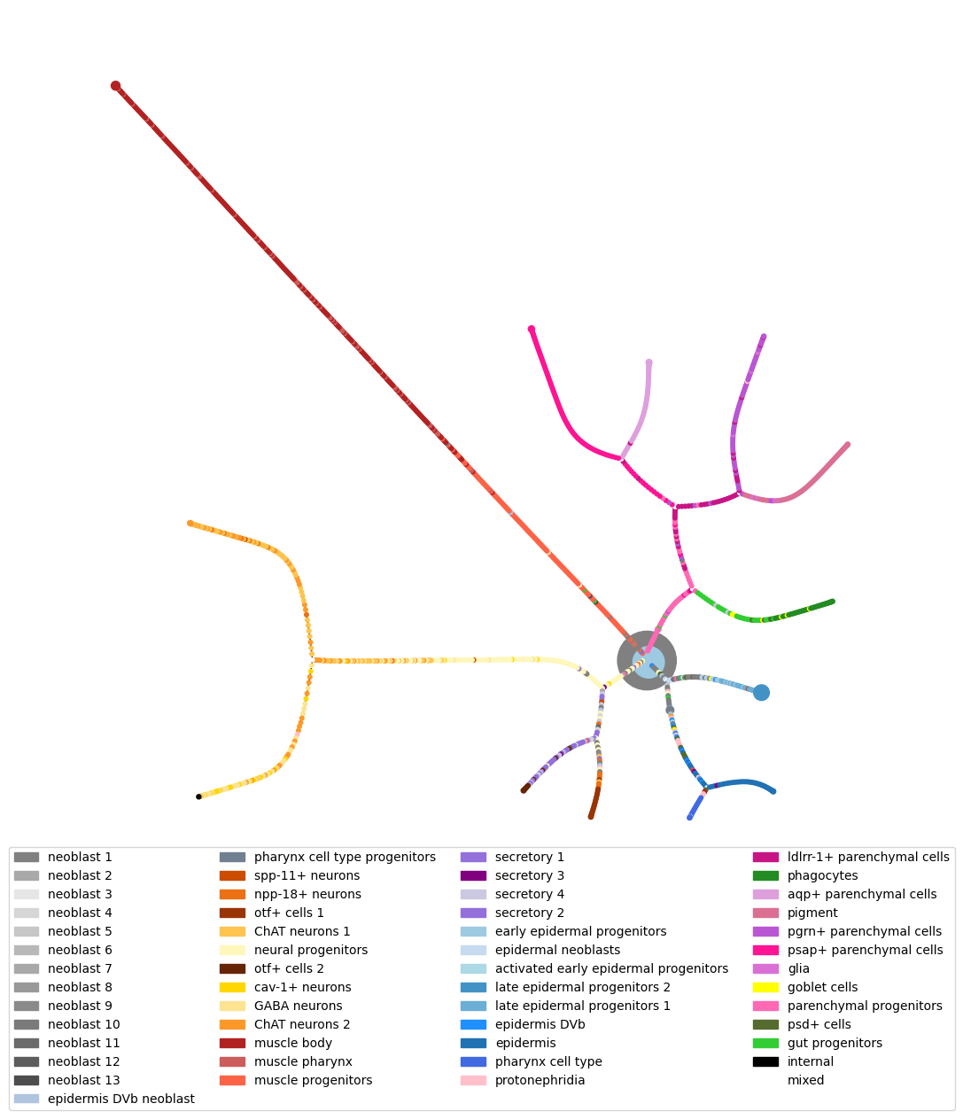
This can then be plotted. Points are coloured by labels, if a plotted
node is a collection of data points then colour_threshold controls
when to colour this node by the majority type of data point (colour by
majority if proportion of majority is greater than colour_threshold),
else, if there is no majority node, it is plotted white.
Layouts, node settings and others can also be changed. See the documentation for details of this.
tree = eb.ConstructTree(zeta, epsilon=0.2)
tree.fit()
Performing clustering...
Calculating branch lengths...
Constructing tree...
<pyemb.hc.ConstructTree at 0x7a1014496170>
fig = tree.plot(labels = labels,
                colours = colors,
                add_legend = True,
                move_legend = (.5,-.25),
                prog = 'twopi')
100%|██████████| 250/250 [00:03<00:00, 69.38it/s]
BarnesHut Approximation  took  2.26  seconds
Repulsion forces  took  1.08  seconds
Gravitational forces  took  0.02  seconds
Attraction forces  took  0.01  seconds
AdjustSpeedAndApplyForces step  took  0.12  seconds

References
Plass, M., Solana, J., Wolf, F.A., Ayoub, S., Misios, A., Glažar, P., Obermayer, B., Theis, F.J., Kocks, C. and Rajewsky, N., 2018. Cell type atlas and lineage tree of a whole complex animal by single-cell transcriptomics. Science, 360(6391), p.eaaq1723.
Whiteley, N., Gray, A. and Rubin-Delanchy, P., 2022. Statistical exploration of the Manifold Hypothesis.
Gray, A., Modell, A., Rubin-Delanchy, P. and Whiteley, N., 2024. Hierarchical clustering with dot products recovers hidden tree structure. Advances in Neural Information Processing Systems, 36.