20Newsgroup documents
This sections aims to use the packages functionality on text data. This includes creating a amtrix of tf-idf features, PCA and hierarchical clustering. For this, we will demonstrate on a sample of the 20Newsgroup data. Each document is associated with 1 of 20 newsgroup topics, organized at two hierarchical levels.
Data load
Import data and create dataframe.
df = eb.load_newsgroup()
Data loaded successfully
eb.text_matrix_and_attributes - creates a Y matrix of tf-idf
features. It takes in a dataframe and the column which contains the
data. Further functionality includes: removing general stopwords, adding
stopwords, removing email addresses, cleaning (lemmatize and remove
symbol, lowercase letters) and a threshold for the min/max number of
documents a word needs to appear in to be included.
Y, attributes = eb.text_matrix_and_attributes(df, 'data', remove_stopwords=True, clean_text=True,
                                    remove_email_addresses=True, update_stopwords=['subject'],
                                    min_df=5, max_df=len(df)-1000)
(n,p) = Y.shape
print("n = {}, p = {}".format(n,p))
n = 5000, p = 12804
Perform dimension selection using Wasserstein distances, see Whiteley et al., 2022 for details.
ws, dim = eb.wasserstein_dimension_select(Y, range(40), split=0.5)
print("Selected dimension: {}".format(dim))
Selected dimension: 28
PCA and tSNE
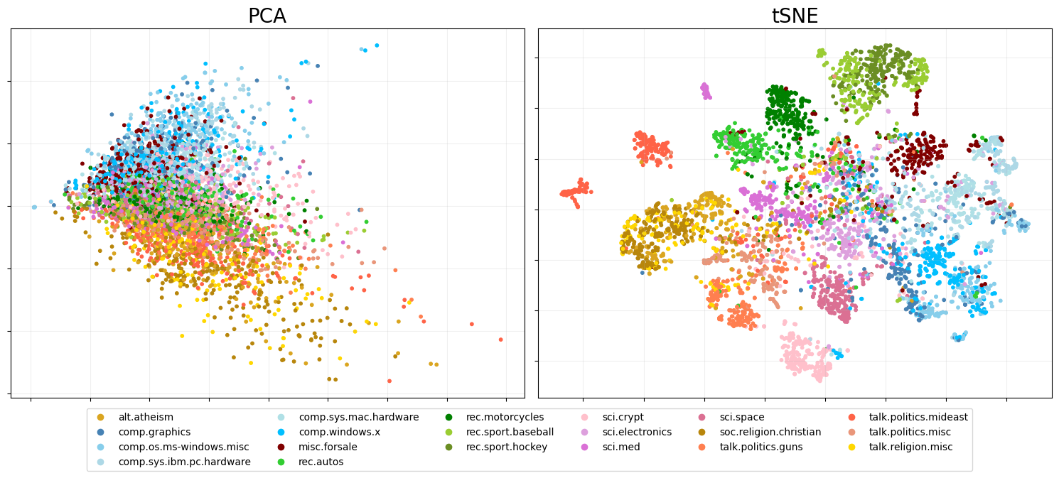
Now we perform PCA Whiteley et al., 2022.
zeta = p**-.5 * eb.embed(Y, d=dim, version='full')
Apply t-SNE.
from sklearn.manifold import TSNE

tsne_zeta = TSNE(n_components=2, perplexity=30).fit_transform(zeta)
Colours dictionary where topics from the same theme have different shades of the same colour
target_colour = {'alt.atheism': 'goldenrod',
                 'comp.graphics': 'steelblue',
                 'comp.os.ms-windows.misc': 'skyblue',
                 'comp.sys.ibm.pc.hardware': 'lightblue',
                 'comp.sys.mac.hardware': 'powderblue',
                 'comp.windows.x': 'deepskyblue',
                 'misc.forsale': 'maroon',
                 'rec.autos': 'limegreen',
                 'rec.motorcycles': 'green',
                 'rec.sport.baseball': 'yellowgreen',
                 'rec.sport.hockey': 'olivedrab',
                 'sci.crypt': 'pink',
                 'sci.electronics': 'plum',
                 'sci.med': 'orchid',
                 'sci.space': 'palevioletred',
                 'soc.religion.christian': 'darkgoldenrod',
                 'talk.politics.guns': 'coral',
                 'talk.politics.mideast': 'tomato',
                 'talk.politics.misc': 'darksalmon',
                 'talk.religion.misc': 'gold'}
Plot PCA on the LHS and PCA + t-SNE on the RHS
pca_fig = eb.snapshot_plot(
    embedding = [zeta[:, :2],tsne_zeta],
    node_labels = df['target_names'].tolist(),
    c = target_colour,
    title = ['PCA','tSNE'],

    add_legend=True,
    max_legend_cols = 6,
    figsize = (15,6),
    move_legend = (.5,-.15),
    # tick_labels = True,
    # Apply other matplotlib settings
    s=10,
)
plt.tight_layout()

Hierarchical clustering with dot products, Gray et al., 2024
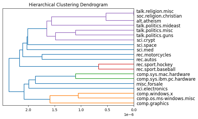
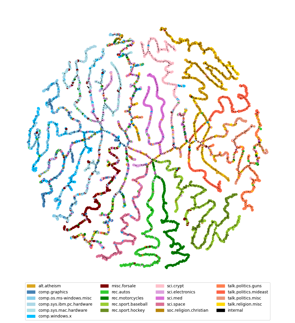
First we do HC for the centroids of each topic and plot the dendrogram. Then we do HC on the whole dataset and visualise the output tree.
On centroids
Find centroids
idxs = [np.where(np.array(df['target']) == t)[0]
        for t in sorted(df['target'].unique())]
t_zeta = np.array([np.mean(zeta[idx, :], axis=0) for idx in idxs])
Topic HC clustering
t_dp_hc = eb.DotProductAgglomerativeClustering()
t_dp_hc.fit(t_zeta);
Plot dendrogram
plt.title("Hierarchical Clustering Dendrogram")
eb.plot_dendrogram(t_dp_hc, dot_product_clustering=True, orientation='left',
                   labels=sorted(df['target_names'].unique()))
plt.show()

On documents
dp_hc = eb.DotProductAgglomerativeClustering()
dp_hc.fit(zeta);
Use construct tree graph from hierarchical clustering, epsilon is set to zero as we don’t want to prune the tree.
tree = eb.ConstructTree(model= dp_hc, epsilon=0)
tree.fit()
Constructing tree...
<pyemb.hc.ConstructTree at 0x74ee20fbf280>
tree.plot(labels = list(df["target_names"]), colours = target_colour, node_size=25, forceatlas_iter=100)
100%|██████████| 100/100 [00:11<00:00, 9.00it/s]
BarnesHut Approximation  took  6.12  seconds
Repulsion forces  took  4.49  seconds
Gravitational forces  took  0.04  seconds
Attraction forces  took  0.03  seconds
AdjustSpeedAndApplyForces step  took  0.20  seconds

References
Whiteley, N., Gray, A. and Rubin-Delanchy, P., 2022. Statistical exploration of the Manifold Hypothesis.
Gray, A., Modell, A., Rubin-Delanchy, P. and Whiteley, N., 2024. Hierarchical clustering with dot products recovers hidden tree structure. Advances in Neural Information Processing Systems, 36.